Introduction

Introduction

An all in one knowledge base of machine learning topics. I have documented the most important parts of many difference courses I have taken from coursera and udemy in hopes of having a good reference page to go back to.

Most of this page uses the python programming language.

Environment Setup

Before starting any new project it is highly recommended that you create virtual python environments for each project so that you have isolated python environments for each project. I use pipenv

• First install pipenv via a command such as:

pip install pipenv

• Now go to the folder where you will create a new python virtual environment and run

pipenv shell

This creates a Pipfile. Now you can install dependencies via pipenv install. For example:

pipenv install numpy pandas matplotlib

KL Divergence

Let’s say you have two coins, a Nickel and a Dime. They might be unfair (meaning that they might not be heads or tails 50% of the time).

You are running a gambling ring. People come up to you, and they bet on whether the Nickel will come up heads or tails when you flip it. If they bet a dollar per flip, how much should they win if they get it right?

You might think they should just win a dollar any time they are right, and lose a dollar any time they are wrong. But what if the Nickel is unfair? What if it comes up heads 80% of the time? Smart bettors will take a lot of your money by betting heads. So you might want to change the payout so that if they bet heads and get it right, they only win $0.25. And if they bet tails and get it right, they win $4. This way, on average, you will win as much as you lose. And the bettors don’t have an advantage or disadvantage by betting heads or tails.

What does this have to do with KL divergence? Well let’s say that you can’t flip the Nickel yourself to figure out how often it comes up heads. How do you decide what each bet should be? You could just default to the “bet a dollar, win a dollar” setup. Or you could flip the Dime. Let’s say that you flip the dime a thousand times, and see how often it comes up heads or tails. You could use the Dime to guess how the Nickel will behave.

KL Divergence is a measure of how “good” the Dime is at predicting what the Nickel will do. If the KL Divergence is 0, then the Dime is a perfect predictor of the Nickel - they both come up heads or tails at the same rate. But if the Dime is a bad predictor of the Nickel’s behavior, the KL Divergence will be large. This basically means that if you were using the Dime to make your decisions, and you replaced it by actually flipping the Nickel a lot and seeing what it does, you would gain a bunch of information and be able to set better odds (odds that don’t allow smart bettors to take your money).

More generally, KL Divergence says that if I use distribution A to predict the behavior of some random process, and the process actually happens with distribution B, how much worse am I doing by using A as an estimate than if I had access to B directly?

Scatter Plot

Scatter plots draws points without lines connecting them.

import matplotlib.pyplot as plt

X = [1, 2, 3, 4]
Y = [2, 4, 6, 8]

plt.scatter(X, Y, color = 'red')

Plot Plot

Plots draws lines between points.

import matplotlib.pyplot as plt

X = [1, 2, 3, 4]
Y = [2, 4, 6, 8]

plt.plot(X, Y, color = 'red')

Boxplot

A boxplot is a way to show the spread and centers of a data set.

import seaborn as sns
import pandas as pd
import matplotlib.pyplot as plt

filename = 'foo_train.csv'
df_train = pd.read_csv(filename)

# With matplotlib all data

df_train.boxplot()

# With seaborn, box plot overallqual/saleprice
var = 'OverallQual'
data = pd.concat([df_train['SalePrice'], df_train[var]], axis=1)
f, ax = plt.subplots(figsize=(8, 6))
fig = sns.boxplot(x=var, y="SalePrice", data=data)
fig.axis(ymin=0, ymax=800000)

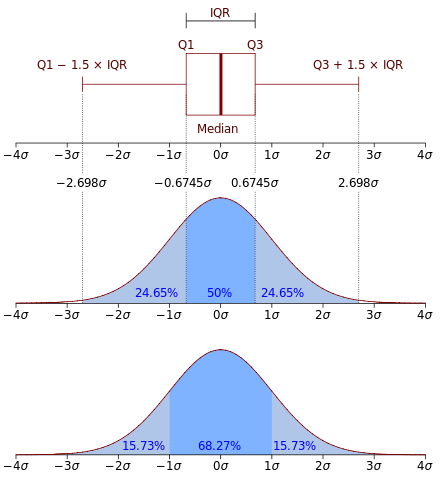
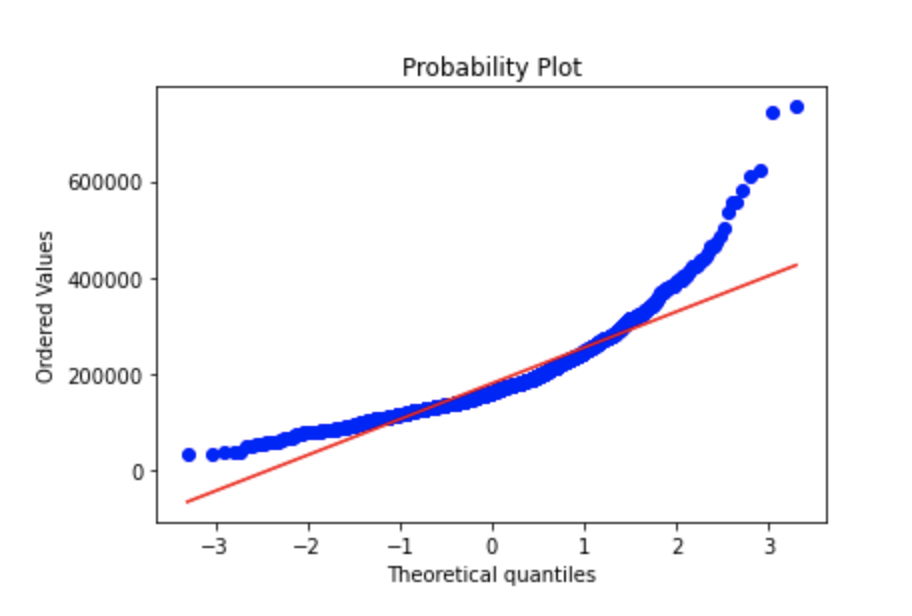
Q Q Plot

In statistics, a Q–Q plot is a probability plot, which is a graphical method for comparing two probability distributions by plotting their quantiles against each other.

Basically, a way to visually see if the data is normally distributed. full details

A normal distribution’s qq plot looks like:

Your data might have a skew, in which case your graph can look like:

import matplotlib.pyplot as plt
from scipy import stats

fig = plt.figure()
res = stats.probplot(train['SalePrice'], plot=plt)
plt.show()

Log tranformation might be required when dealing with skewed data - The log transformation can be used to make highly skewed distributions less skewed. This can be valuable both for making patterns in the data more interpretable and for helping to meet the assumptions of inferential statistics.

Correlation Matrix

Basically a covariance matrix. It is a matrix in which i-j position defines the correlation between ith and jth parameters.

import seaborn as sns
import pandas as pd
import matplotlib.pyplot as plt

filename = 'foo_train.csv'
df_train = pd.read_csv(filename)

corrmat = df_train.corr()
f, ax = plt.subplots(figsize=(12, 9))
sns.heatmap(corrmat, vmax=.8, square=True)
# or
sns.heatmap(corrmat,ax= ax, cmap='coolwarm')

Lets say you want to find the top k variables correlated to your label variable.

#saleprice correlation matrix
k = 10 #number of variables for heatmap
cols = corrmat.nlargest(k, 'SalePrice')['SalePrice'].index
cm = np.corrcoef(df_train[cols].values.T)
sns.set(font_scale=1.25)
hm = sns.heatmap(cm, cbar=True, annot=True, square=True, fmt='.2f', annot_kws={'size': 10}, yticklabels=cols.values, xticklabels=cols.values)
plt.show()

credits

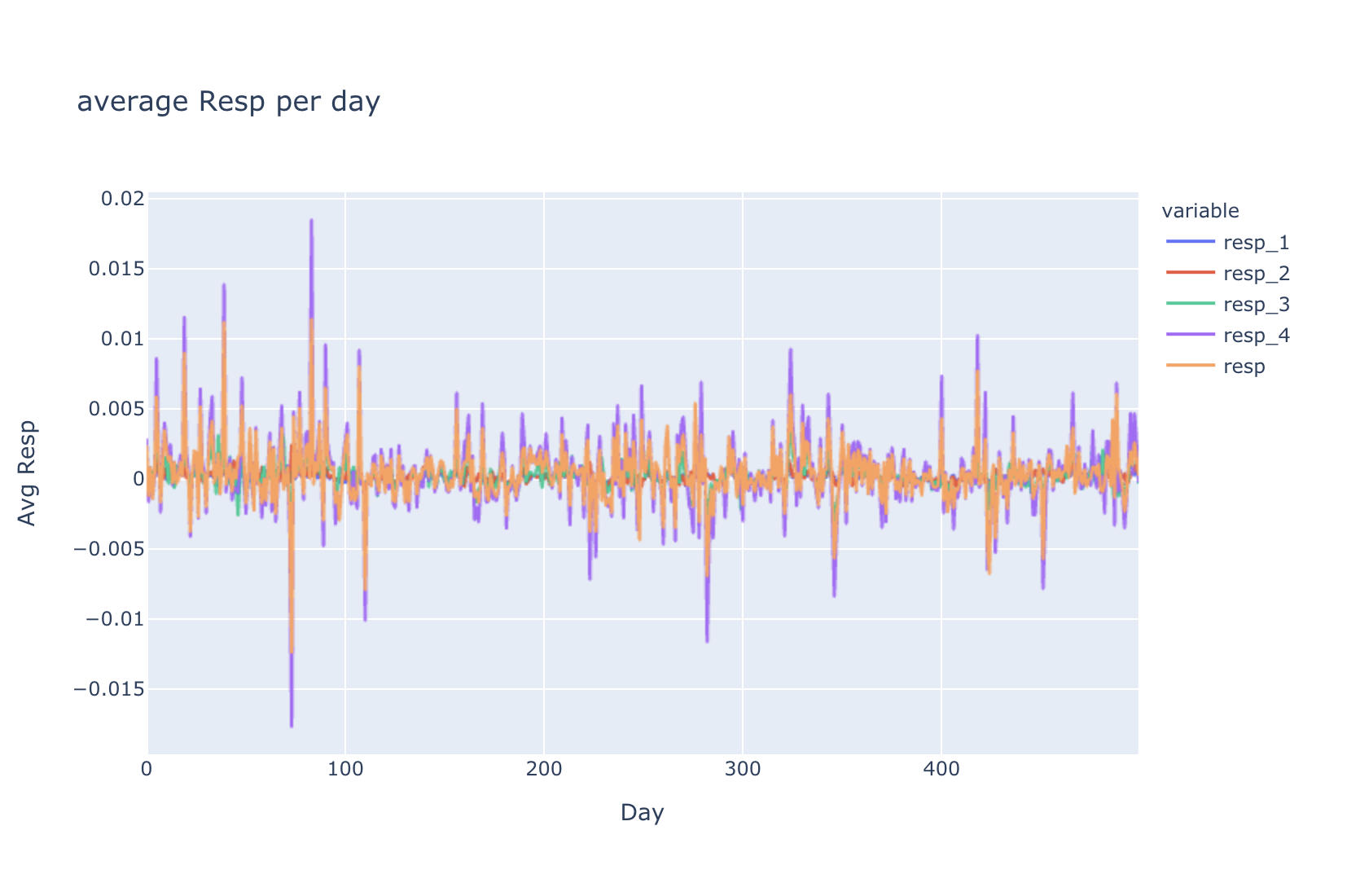
Average Over Time

The example below uses a pandas dataframe and date is a integer from 0 to 500.

fig = px.line(df.groupby('date')[['resp_1', 'resp_2', 'resp_3', 'resp_4','resp']].mean(),
              x= df.groupby('date')[['resp_1', 'resp_2', 'resp_3', 'resp_4','resp']].mean().index,
              y= ['resp_1', 'resp_2', 'resp_3', 'resp_4','resp'],
              title= '\naverage Resp per day')
fig.layout.xaxis.title = 'Day' 
fig.layout.yaxis.title = 'Avg Resp'
fig.show()

Read from csv

Your have a comma separated values file such as:

2019,Acura,RDX, FWD w/Advance Pkg,$45,500,22 mpg City/28 mpg Hwy
2019,Acura,RDX, FWD w/A-Spec Pkg,$43,600,22 mpg City/27 mpg Hwy
2019,Acura,RDX, FWD,$37,400,22 mpg City/28 mpg Hwy

import pandas as pd

filename = 'foo.csv'
pd.read_csv(filename)

Read from json

You have multiple json objects in a file separated by a newlines such as:

{"year": 2007, "make": "Volkswagen", "model": "New", "trim": "'Beetle Convertible 2.5 2dr Convertible (2.5L 5cyl 6A)'", "engine_type": "gas", "no_doors": 2, "review_year": "09/18/11", "years_owned": 4, "comment": " I've had my Beetle Convertible for over 4.5 years andhave been overall happy with the car. It is a compact convertible.Don't expect a big trunk or having tall people in the back seat."}
{"year": 2007, "make": "Volkswagen", "model": "New", "trim": "'Beetle Convertible 2.5 PZEV 2dr Convertible (2.5L 5cyl 6A)'", "engine_type": "gas", "no_doors": 2, "review_year": "07/07/10", "years_owned": 3, "comment": " We bought the car new in 2007 and are generally satisfied. Mechanically the car has been good but build quality needs improvement except for the paint job which is the best I have ever seen.  Problems we have had are: 1. Three headlight bulbs replaced. 2. Entire locking mechanism for power convertible top had to be replaced. 3. Coolant temperature switch replaced. 4. Four trunk pistons failed with the fifth now broken. 5. Seat belt retainer bezel broken off and replaced.  Fuel mileage is average that is 25 around town - less if air running and about 30 mpg at 65 mph if air not running.  Trunk space is inadequate and simple repair under the hood is difficult and expensive."}
{"year": 2007, "make": "Volkswagen", "model": "New", "trim": "'Beetle Convertible Triple White PZEV 2dr Convertible (2.5L 5cyl 6A)'", "engine_type": "gas", "no_doors": 2, "review_year": "10/19/09", "years_owned": 2, "comment": " I adore my New Beetle. Even though I'm a male, I get compliments from my other guy friends, especially after they've driven it. Convertible a must! The only problem I've had was the wiring harness shorted. Fortunately, the car is still under warranty, and will be back to running soon!"

import json
import pandas as pd

filename = 'foo.txt'
object_list = []
with open(filename, 'r') as f:   
    object_list = [json.loads(line) for line in f.readlines()]
dataframe = pd.DataFrame(object_list)

Dataframe to Numpy Array

import pandas as pd

df= pd.read_csv('file.csv')
numpy_arr = df.values

Or for specific values in the dataframe:

import pandas as pd

df = pd.read_csv('file.csv')
X = df.iloc[:,:-1].values
Y = df.iloc[:,-1].values

Replacing Missing Values

Most datasets have missing data. Use scikit-learn’s imputer class to fill the missing values. Almost always use the mean strategy. It just works!

First read the data. How to read csv to numpy

from sklearn.impute import SimpleImputer

imputer = SimpleImputer(missing_values=np.nan, strategy='mean')
imputer.fit(X[:,1:3])
X[:,1:3] = imputer.transform(X[:,1:3])

Encoding Categorical Data

OneHotEncoder

Categorical data or variables represent types of data which may be divided into groups. For example, race, sex, educational level.

This data needs to be represented as numerical values for our machine learning models to process. This is what encoding does.

Ex: You have a variable which represents country names:

[[France 44.0 72000.0
Italy 27.0 48000.0
Spai 30.0 54000.0]]

Apply one hot encoding as follows:

from sklearn.compose import ColumnTransformer
from sklearn.preprocessing import OneHotEncoder
ct = ColumnTransformer(transformers=[('encoder', OneHotEncoder(), [0])], remainder='passthrough')
X = np.array(ct.fit_transform(X))

Note: the ColumnTransformer gets passed the index via [0] of the column we want to encode.

Result:

[[1.0 0.0 0.0 44.0 72000.0
0.0 0.0 1.0 27.0 48000.0
0.0 1.0 0.0 30.0 54000.0]]

Encoded data does not need to be feature scaled (for example standardized scaling)

LabelEncoder

If your data is binary, such as True and False then apply the following encoding.

Y: [Yes Yes No No]

from sklearn.preprocessing import LabelEncoder
le = LabelEncoder()
Y = le.fit_transform(Y)

Result:

[1 1 0 0]

Splitting Datasets Into Training Test Sets

For the most part use 20% as the test size.

from sklearn.model_selection import train_test_split
X_train, X_test, Y_train, Y_test = train_test_split(X,Y, test_size=0.2, random_state=1)

Feature Scaling

Your variables if not scaled can overpower your machine learning models. For example, age if usually from 1 to 100, while car price can be from 10000 to 200000. In this instance your model will be skewed by such large numbers in the variable car price.

To solve this problem, do feature scaling.

from sklearn.preprocessing import StandardScaler
sc = StandardScaler()
X_train[:,3:] = sc.fit_transform(X_train[:,3:])
X_test[:,3:] = sc.fit_transform(X_test[:,3:])
# sc.inverse_transform to reverse the values back.

In this case we standardized the values, meaning:

new_value = (value - mean) / (standard_deviation)

Something like this:

[[0.0 0.0 1.0 38.77777777777778 52000.0]
 [0.0 1.0 0.0 40.0 63777.77777777778]
 [1.0 0.0 0.0 44.0 72000.0]
 [0.0 0.0 1.0 38.0 61000.0]
 [0.0 0.0 1.0 27.0 48000.0]
 [1.0 0.0 0.0 48.0 79000.0]
 [0.0 1.0 0.0 50.0 83000.0]
 [1.0 0.0 0.0 35.0 58000.0]]

Turns into this

 [[0.0 0.0 1.0 -0.1915918438457856 -1.0781259408412427]
 [0.0 1.0 0.0 -0.014117293757057902 -0.07013167641635401]
 [1.0 0.0 0.0 0.5667085065333239 0.6335624327104546]
 [0.0 0.0 1.0 -0.3045301939022488 -0.30786617274297895]
 [0.0 0.0 1.0 -1.901801144700799 -1.4204636155515822]
 [1.0 0.0 0.0 1.1475343068237056 1.2326533634535488]
 [0.0 1.0 0.0 1.4379472069688966 1.5749910381638883]
 [1.0 0.0 0.0 -0.7401495441200352 -0.5646194287757336]]

We do not standardize one-hot encoded variables.

Min Max scaler example

 from sklearn.preprocessing import MinMaxScaler

 def normalize():
    min_max_scaler = MinMaxScaler()
    column_names_to_normalize = ['loan_amount_000s', 'applicant_income_000s','minority_population']
    x = df[column_names_to_normalize].values
    x_scaled = min_max_scaler.fit_transform(x)
    df_temp = pd.DataFrame(x_scaled, columns=column_names_to_normalize, index=df.index)
    df[column_names_to_normalize] = df_temp

Assumptions of Linear Regression

• Linearity: relationship between X and the mean of Y is linear
• Homoscedasticity: variance of residual is the same for any value of X.
• Independence: observations are independent of each other
• Normality: for any fixed value of X, Y is normally distributed.

Simple Linear Regression

Remember y = mx + b ? Linear regression finds the most optimal parameters m and b that fit a set of points (x,y)

Ex:

Given these points:

(0,0)
(1,2)
(2,4)
(3,6)
(4,8)

By eyeballing the values, We know the equation is y = 2x. Our regression model should find this answer.

After loading the data, replacing missing values, encoding categorical data, splitting datasets into test and train sets and feature scaling, you are ready to run a simple linear regression

from sklearn.linear_model import LinearRegression
from sklearn.metrics import mean_squared_error, r2_score

regressor = LinearRegression()
regressor.fit(X_train, y_train)

# predict values
y_pred = regressor.predict(X_test)

# The mean squared error
print('Mean squared error: %.2f'
      % mean_squared_error(y_test, y_red))
# The coefficient of determination: 1 is perfect prediction
print('Coefficient of determination: %.2f'
      % r2_score(y_test, y_pred))

Multivariate Regression

Not all models take 1 input to predict 1 output. This type of model takes multiple inputs to predict one output.

y = b0 + b1x1 + b2x2 + ... + bnxn

The steps are the same as simple linear regression.

Polynomial Regression

If the data doesnt have a linear relationship, using polynomial regression might increase accuracy.

\[y = b_{0} + b_{1}x_{1} + b_{2}x_{1}^2 + … + b_{n}x_{1}^n\]

After loading the data, replacing missing values, encoding categorical data, splitting datasets into test and train sets and feature scaling, you are ready to run a polynomial regression

from sklearn.linear_model import LinearRegression
from sklearn.preprocessing import PolynomialFeatures

poly_reg = PolynomialFeatures(degree = 4)
# this line transforms your y = mx + b into y = b0 + b1x1 + b2x1^2 + b3x1^3 + b4x1^4
X_poly = poly_reg.fit_transform(X)
# pass X_poly into a linear regression , that's just how it works
lin_reg_2 = LinearRegression()
lin_reg_2.fit(X_poly,Y)

Support Vector Regression

The key to SVR is that it uses a margin of error, e-insensitive tube, that we allow our model to have. Anything that falls inside that margin of error, we will disregard the error from those points.

from sklearn.svm import SVR
regressor = SVR(kernel = 'rbf')
regressor.fit(X, y)

Decision Trees

First: loading the data, replacing missing values, encoding categorical data, splitting datasets into test and train sets BUT NO NEED TO APPLY feature scaling because they split the data through different nodes of the tree instead of using some equations like the linear regression models.

import matplotlib.pyplot as plt 
from sklearn.tree import DecisionTreeRegressor

regressor = DecisionTreeRegressor(random_state = 0)
regressor.fit(X, y)

regressor.predict([[6.5]])

#Visualize the decision tree results
X_grid = np.arange(min(X), max(X), 0.01)
X_grid = X_grid.reshape((len(X_grid), 1))
plt.scatter(X, y, color = 'red')
plt.plot(X_grid, regressor.predict(X_grid), color = 'blue')
plt.title('Truth or Bluff (Decision Tree Regression)')
plt.xlabel('Position level')
plt.ylabel('Salary')
plt.show()

Random Forest

Random forest is a version of ensemble learning (the process by which multiple models, such as classifiers are strategically generated and combined to solve a particular computational intelligence problem)

from sklearn.ensemble import RandomForestRegressor

regressor = RandomForestRegressor(n_estimators = 10, random_state = 0)
regressor.fit(X, y)

regressor.predict([[6.5]])

# Visualize the results 
X_grid = np.arange(min(X), max(X), 0.01)
X_grid = X_grid.reshape((len(X_grid), 1))
plt.scatter(X, y, color = 'red')
plt.plot(X_grid, regressor.predict(X_grid), color = 'blue')
plt.title('Truth or Bluff (Random Forest Regression)')
plt.xlabel('Position level')
plt.ylabel('Salary')
plt.show()

Logistic Regression

Used to solve classification problems. For example, given input data, solves for whether the label is true or false, or zero or one.

\[S(x) = \frac{1}{1+e^{-x}}\]

Applying feature scaling although not necessary, will improve training performance.

from sklearn.linear_model import LogisticRegression
from sklearn.metrics import accuracy_score

classifier = LogisticRegression(random_state = 0)
classifier.fit(X_train, y_train)

# use sc.transform if you did feature scaling.
print(classifier.predict(sc.transform([[30,87000]])))

# accuracy score
accuracy_score(y_test, y_pred)

Evaluate your algorithm with a confusion matrix

K Nearest Neighbors

KNN is a simple easy to implement supervised machine learning algorithm that can be used to solve classification and regression problems

Based on comparing input features of datasets by their distances and the closest points are categorized into the same groups. In the most basic approach, something like the manhattan distances can be used.

from sklearn.neighbors import KNeighborsClassifier

classifier = KNeighborsClassifier(n_neighbors = 5, metric = 'minkowski', p = 2)
classifier.fit(X_train, y_train)

print(classifier.predict(sc.transform([[30,87000]])))

Evaluate your algorithm with a confusion matrix

Support Vector Machine

Some intuition in support vector regression

from sklearn.svm import SVC

classifier = SVC(kernel='linear')

classifier.fit(X_train, y_train)
print(classifier.predict(sc.transform([[30,87000]])))

If data is not linearly separable use a different kernel.

from sklearn.svm import SVC
classifier = SVC(kernel = 'rbf', random_state = 0)
classifier.fit(X_train, y_train)
print(classifier.predict(sc.transform([[30,87000]])))

Kernels

Decision Tree Classifier

from sklearn.tree import DecisionTreeClassifier
classifier = DecisionTreeClassifier(criterion = 'entropy', random_state = 0)
classifier.fit(X_train, y_train)
# predict
print(classifier.predict(sc.transform([[30,87000]])))

Random Forest Classifier

from sklearn.ensemble import RandomForestClassifier
classifier = RandomForestClassifier(n_estimators = 10, criterion = 'entropy', random_state = 0)
classifier.fit(X_train, y_train)
#predict
print(classifier.predict(sc.transform([[30,87000]])))

Binary Classifier Neural Network Using Tensorflow and Keras

After loading the data, replacing missing values, encoding categorical data, splitting datasets into test and train sets and feature scaling, you are ready to create a neural network to make predictions.

The last layer has a sigmoid activation function for binary classification.

import tensorflow as tf
from tensorflow.keras import layers
from tensorflow.keras import optimizers
from tensorflow.keras import Sequential
from tensorflow.keras import Dense

def create_model(input_size):
    model = Sequential()
    model.add(layers.Dense(100, activation=tf.nn.relu, kernel_initializer='uniform', input_shape=(input_size,)))
    model.add(layers.Dense(75, activation=tf.nn.relu))
    model.add(layers.Dense(50, activation=tf.nn.relu))
    model.add(layers.Dense(25, activation=tf.nn.relu))
    model.add(layers.Dense(1, activation=tf.nn.sigmoid))

    optimizer = optimizers.RMSprop(lr=0.0001)
    model.compile(loss='binary_corssentropy', optimizer=optimizer, metrics=['accuracy'])

    return model

train it by calling:

model.fit(x_train, y_labels)

predict:

model.predict(test_data)

Callbacks

When calling fit it might be useful to use callbacks to do early stopping, save the best epoch’s weights or reduce learning rate on plateau.

mcp_save = ModelCheckpoint('01012021_v1.hdf5', save_best_only=True, monitor='val_AUC', mode='min')
rlr = ReduceLROnPlateau(monitor = 'val_AUC', factor = 0.1, patience = 3, verbose = 0, min_delta = 1e-4, mode = 'max')
earlyStopping = EarlyStopping(monitor='val_loss', patience=20, verbose=0, mode='min')
model.fit(X_train, Y_train, epochs = 100, batch_size = batch_size, verbose = 1, callbacks=[earlyStopping, mcp_save, rlr], validation_data=(X_test,Y_test))

R Squared and Adjusted R Squared

R squared, the coefficient of determination, shows how well data points fit a curve or line. Adjusted R squred also indicates how well data points fit a curve or line but adjusts for the number of data points in the model.

The closer R squared (or adjusted R squared) is to 1 the better the model fits.

If you add more useless data points to a model, the adjusted R squred will decrease, while if you add more useful data points, adjusted R squred will increase.

\[R^2 = 1 - \frac{RSS}{TSS}\] where: RSS = sum of square of residuals, TSS = total sum of squares

\[R_{adj}^2 = 1 - \frac{(1-R^2)(n-1)}{n-k-1}\] where: n is the number of points in your data sample, k is the number of independent variables in your model.

read it in detail herehere

Confusion Matrix

Also known as an error matrix, is a specific table layout that allows visualization of the performance of classification algorithms.

from sklearn.metrics import confusion_matrix

y_true = [2, 0, 2, 2, 0, 1]
y_pred = [0, 0, 2, 2, 0, 2]
confusion_matrix(y_true, y_pred)

array([[2, 0, 0],
       [0, 0, 1],
       [1, 0, 2]])

Seq2seq and Attention

This great blog by Leva Voita does a better job than I ever will.

Libraries and Tools

There are a great number of libraries and tools out there. Here I document some of the ones I have found very useful.

• huggingface transformers - Provides thousands of pretrained models to perform tasks on texts such as classification, information extraction, question answering, summarization, translation, text generation, etc in 100+ languages. Its aim is to make cutting-edge NLP easier to use for everyone.

• pycaret - PyCaret is an open-source, low-code machine learning library in Python that automates machine learning workflows. It is an end-to-end machine learning and model management tool that speeds up the experiment cycle exponentially and makes you more productive.

• hyperopt or optuna - Hyperparameter optimization

Public Datasets

• Document images with labels

Sources

Resources used for this page

• Machine Learning A-Z: Hands-On Python & R In Data Science by Kirill Eremenko
• Deep Learning Specialization by Andrew Ng
• The Data Science Course 2020: Complete Data Science Bootcamp by Kirill Eremenko
• Artificial Intelligence: Reinforcement Learning in Python by Lazy Programmer
• Advanced AI: Deep Reinforcement Learning in Python by Lazy Programmer
• Kaggle