Population vs Sample

A population is the entire group that you want to draw conclusions about. In other words, you have all the data available.
A sample is a specific group that you will collect data from. Statistics mostly uses samples because capturing all data is improbable or impossible.

Mean vs Median vs Mode

Mean: the summation of n numbers divided by n.

\[\mu = ( \frac{1}{n} \sum_{i}^{n} x_{i} )\]

Median: middle number in a sorted, ascending or descending list of numbers.

If n is even:

\[Med(X) = X[\frac{n}{2}]\]

If n is odd:

\[Med(X) = \frac{X[\frac{n-1}{2} + X[\frac{n+1}{2}]]}{2}\]

Mode is the value that appears most often in a set of values.

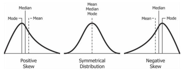
Skewness

For normally distributed data, the skewness should be about zero. For unimodal continuous distributions, a skewness value greater than zero means that there is more weight in the right tail of the distribution. The function skewtest can be used to determine if the skewness value is close enough to zero, statistically speaking.

Basically skewness is a measure of symmetry or lack of symmetry. It indicates whether the data is concentrated on one side.

If mean > median, this is a positive or right skew.
If mean = median = mode, there is no skew (distribution is semetrical)
If mean < median, this is negative or left skew.

skewness_img

skewness in wikipedia

Many classical statistical tests and intervals depend on normality assumptions. Significant skewness and kurtosis clearly indicate that data are not normal. If a data set exhibits significant skewness or kurtosis we might apply some type of transformation to make the data normal.

from scipy.stats import skew

skew([1, 2, 3, 4, 5])
# Result: [0.0]

skew([2, 8, 0, 4, 1, 9, 9, 0])
# Result: [0.2650554122698573]

Apply Box Cox transform to skewed features

from scipy.special import boxcox1p

skewed_features = skewness.index
lam = 0.15
for feat in skewed_features:
    all_data[feat] = boxcox1p(all_data[feat], lam)

Kurtosis

Kurtosis is a measure of the “tailedness” of the distribution. That is, datasets with high kurtosis tend to have heavy tails, or outliers. Data sets with low kurtosis tend to have light tails, or lack of outliers.

The kurtosis for a standard normal distribution is 3.

Variance

The average of squared differences from the mean.

Variance can be calculated for a population or for a sample.

For a population:

\[\sigma^2 = \frac{1}{n}\sum_{i}^{n} (x_{i} - \mu)^2\]

For a sample:

\[S^2 = \frac{1}{n-1}\sum_{i}^{n} (x_{i} - \bar{x})^2\]

Standard Deviation

For a population:

\[\sigma = \sqrt{\sigma^2}\]

For a sample:

\[S = \sqrt{S^2}\]

Coefficient of Variation

Also known as the relative standard deviation.

\[CV = \frac{\sigma}{\mu}\]

Comparing the standard deviation of two datasets is meaningless, however, comparing their coefficient of variation is not

Helps us compare variability across multiple datasets.

Covariance

Covariance is the statistical measure of correlation.

Formula to calculate covariance between two variables

for a population

\[\sigma_{xy} = \frac{\sum_{i=1}^N (x_{i}-\mu_{x})*(y_{i}-\mu_{y})}{N}\]

for a sample

\[S{xy} = \frac{\sum_{i=1}^N (x_{i}-\bar{x})*(y_{i}-\bar{y})}{N-1}\]

Covariance gives a sense of direction.

If > 0, the two variables move together.
If < 0. the two variables move in opposite directions.
If = 0, the two variables are independent.

The problem with Covariance is the number is not easy to interpret, so we use the correlation coefficient

Correlation Coefficient

\[r = \frac{Cov(x,y)}{Stdev(x)*Stdev(y)}\]

The closer to 1 the more correlated the variables are.
The closer to 0 means the variables are indepenedent of each other.
We can have a negative correlation from 0 to -1. Ex: A company selling ice cream and another selling umbrellas. They are in some sense exact opposites since when one company makes money the other doesn’t.

Correlation does not imply causation

How to plot a correlation maxtrix

Central Limit Theorem

If you take a lot of samples from a population, their sample mean distribution approaches a normal distribution as the sample size gets larger. Specially true if sample size is over 30.

Ex:

Draw 6 samples out a population. Their means are as follows:

If we create a new dataset based on these values, then they form a normal distribution. This is the basis of the central limit theorem.