Algebra of Sets
Algebra of Sets
In Probability the words set and event are interchangeable.
- \(\Omega\) denotes the full sample space. So \(P(\Omega)=1\).
- \(\emptyset\) denotes the null or empty set.
- \(A \subset B\) means A is a subset of B.
- \(A \cup B\) is the union of A and B.
- \(A \cap B\) is the intersection of A and B.
- \(A^{‘}\) is the complement of A.
Lets break this down.
- \(A \cap B\) is the same as saying A has occured and B has occured at the same time.

- \(A \cup B\) is the same as saying A occured or B occured, or both occured.

Combinatronics
Multiplication Principle
Suppose an experiment E1 has n1 outcomes and for each of these possible outcomes, an experiment E2 has n2 possible outcomes. Then the composite experiment E1E2 that consists of performing first E1 then E2 has n1n2 possible outcomes
Ex: An ice cream shop sells 3 types of flavors and 2 types of cones. How many possible combinations of ice cream can one choose?
Flavors: F1,F2,F3 Cones: C1,C2
So the total combinations are:
(F1,C1),(F1,C2) (F2,C1),(F2,C2) (F3,C1),(F3,C2)
Per our definition, this is the same as n1n2 = (3)*(2) = 6
Permutations
A permutation is a way in which a set or number of things can be ordered or arranged.
Ex: What is the number of permutations of the first four letters of the alphabet a, b, c, d?
Because there is no repetition, choosing one letter reduces the possiblities, so:
4 * 3 * 2 * 1 = 4! = 24
Sampling with Replacement
Occurs when an object is selected and then replaced (placed back) before the next object is selected.
From the previous example, the number of possible four-letter code words if letters are repeated is 4^4 = 256.
Sampling without Replacement
Occurs when an object is not replaced after it has been selected.
\[_{n}P_{r} =\frac{n!}{(n-r)!} \]
Ex: The number of ordered samples of 5 cards that can be drawn without replacement from a 52 card deck.
\[\frac{52!}{(52-5)!}=311875200\]
Arrangements
Filling positions from n different objects.
\[_{n}P_{r} =\frac{n!}{(n-r)!} \]
Ex: What are the number of ways of selecting four letter code words, selecting from the 26 letters of the alphabet?
\[_{26}P_{4} =\frac{26!}{22!}= 358800 \]
Binomial Coefficient
The binomial coefficient \(\binom{n}{k}\) is the number of ways of picking k unordered outcomes from n possibilities.
The equation is:
\[_{n}C_{r}=\binom{n}{k}=\frac{n!}{r!(n-r)!}\]
Ex: How many different pairs can I pick from [1,2,3,4]?
There are six pairs [1,2],[1,3],[1,4],[2,3],[2,4],[3,4]
\[_{4}C_{2}=\frac{4!}{2!(4-2)!}=6\]
Ex: What is the number of possible 5-card hands (in 5-card pocker) drawn from a deck of 52 playing cards?
\[_{52}C_{5}=\binom{52}{5}=\frac{52!}{5!(52-5)!}=2598960\]
What is the probability of event B, that exactly three cards are kings and exactly two hands are queens?
We can select 3 kings in any one of \(\binom{4}{3}\) ways and the queens in any one of \(\binom{4}{2}\) ways. By the multiplication principle:
\[N(B)=\binom{4}{3}\binom{4}{2}\binom{44}{0}\]
where \(\binom{44}{0}\) gives the number of ways in which 0 cards can be selected out of the nonqueens and nonkings (because 5 cards have already been selected). Therefore
\[P(B)=\frac{N(B)}{N(S)}=\frac{\binom{4}{3}\binom{4}{2}\binom{44}{0}}{\binom{52}{5}}=\frac{24}{2598960}=0.0000092\]
Conditional Probability
Conditional probability is the likelihood of an even occuring, assuming a different one has already happened.
\[P(A \mid B)=\frac{P(A \cap B)}{P(B)}\]
Provided P(B) > 0
Ex: A bag contains 25 marbles, of which 10 are yellow, 8 are red and 7 are green. Given that a person takes out a marble at random and is yellow, what is the probability that the next marble randomly picked out of the bag is also yellow? Of the remaining marbles in the bag, 9 are yellow, so the conditional probability is 9/24.
Let A be the event that the first marble taken out is yellow and let B be the event that the second marble is yellow. Then what is the probability that both marbles are yellow?. This is the same as finding \(P(A \cap B)\).
We already know \(P(A) =\frac{10}{25}\) and \(P(B \mid A)=\frac{9}{24}\)
If we plug in into the conditional probability formula \(P(B \mid A)=\frac{P(A \cap B)}{P(A)}\) then we get
\[P(A \cap B)=P(A)P(B \mid A)= \frac{10}{25}\frac{9}{24}\]
The probability that two events, A and B, both occur is given by the multiplication rule:
\[P(A \cap B)=P(B)P(A \mid B)=P(A)P(B \mid A)\]
Provided P(A) > 0
Independent Events
When an occurance of one event does not change the probability of the occurance of the other, then they are said to be independent events. One of example of this is flipping a fair coin. Flipping a coin for the first time doesn’t change the probability of getting a heads or tails the second time because these events are independent.
The mathematical properties for independent events:
\(P(A \mid B)=P(A)\) or \(P(B \mid A)=P(B)\)
and mutually independent if also:
\(P(A \cap B)=P(A)P(B)\)
Also importantly, having indepedence in an original model, does not imply independence in a conditional model. That is, if a new event occurs (conditional model), it might change the assumptions of independence.
Total Probability Theorem
The total probability rule gives you a way of breaking up the calculation of an event that can happen in multiple ways by considering individual probabilities for the different ways that the event can happen.
Ex: Lets say we want to find P(B) given 3 possible scenarios, A1, A2 and A3.
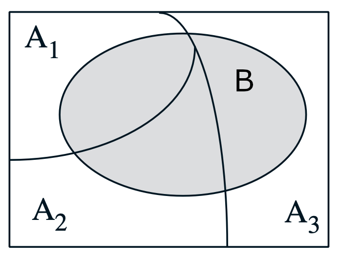
To solve this, partition the sample space and calculate conditional probabilities.
\[P(B) = P(A_{1})P(B \mid A_{1}) + P(A_{2})P(B \mid A_{2}) + P(A_{3})P(B \mid A_{3})\]
Bayes Theorem
Describes the probability of an event based on prior knowledge of conditions that might be related to the event.
\[P(A \mid B)=\frac{P(B \mid A)P(A)}{P(B)}\]
Ex: your boss wants you to do research about what companies are looking for in recent college graduates. Is it good academic performance or experience?
You go over the resume of 200 people that matched the requirements and got the job they applied for. Out of those candidates:
- P(Experience) = 45% … 45% of candiates had prior experience
- P(Good grades) = 60% … 60% of candiates had good grades.
- P(Good grades | experience) = 50% … out of the 45% of candidates that had prior experience, 50% also had good grades.
To find out what companies are looking for, we need to compute the conditional probabiliy of the candidates that had experience provided they had good grades. Using Bayes’ theorem we can compute this as follows:
\[P(Experience \mid Good grades)=\frac{P(Good grades \mid experience)P(Experience)}{P(Good grades)}\]
\[P(Experience \mid Good grades)=\frac{0.5*.45}{0.6}=0.375\]
Because \(P(Experience \mid Good grades)=0.375 < P(Good grades \mid experience)=0.5\)
We can conclude that candidates with experience have a higher likelyhood to get good grades.
Therefore firms are much more likely to get their ideal candidate if they go for someone who’s had experience rather than someone who’s gotten good grades.
Prior and Posterior Probability
Prior probability represents the original probability - what is originally believed before new evidence is introduced.
Posterior probability takes in new evidence into account.
Posterior probability can become prior for a new updated posterior probability as new information arises.
Ex: A school has 60% boys and 40% girls as students. Girls wear trousers or skirts in equal numbers. All boys wear trousers. An observer sees a random student from a distance; all they see is this student wearing trousers. What is the probability this student is a girl?
- P(Girl) = 40% … this is the percentage of girls in the school.
- P(Boy) = 60% … this is the percentage of boys in the school
- P(Trousers | Girl) = 50% … the probability of a student wearing trousers given the student is a girl. Remember, gitls wear trousers or skirts in equal numbers, so 50% of girls wear trousers.
- P(Trousers | Boy) = 100% … all boys wear trousers.
- P(Trousers), or the probability of a randomly picked student wearing trousers can be calculated via the law of total probability
\[P(Trousers)=P(Trousers \mid Girl)P(Girl) + P(Trousers \mid Boy)P(Boy)\]
\[P(Trousers)=0.5 * 0.4 + 1*0.6 = 0.8\]
Therefore, the posterior probability of the observer having spotted a girl given the observed student is wearing trousers can be computed as follows:
\[P(Girl \mid Trousers)=\frac{P(Trousers \mid Girl)P(Girl)}{P(Trousers)}\]
\[P(Girl \mid Trousers)=\frac{0.5 * 0.4}{0.8}=0.25\]
Random Variables
Given a random experiment with an outcome, S, a function X that assigns one and only one real number X(s) = x to each element s in S is called a random variable.
In other words, a random variable is not random. it’s not a variable. It’s just a function from the sample space to the real numbers.
- Functions of random variables are also random variables.
- Random variables can be discrete or continuous.
Ex: a rat is selected at random from a cage and its sex determined. The set of possible outcomes is female and male. Therefore, the outcome space is S = {female, male}. Let X be a function defined on S, our outcome space, such that X(F) = 0 and X(M) = 1. X is a real valued function that has the outcome space S as its domain and the set of real numbers {x: x=0,1} as its range. X is a random variable.
Discrete Random Variables
A discrete random variable has a countable number of possible values. The probability of each value of a discrete random variable is between 0 and 1, and the sum of all the probabilities is equal to 1.
Continuous Random Variables
A continuous random variable is a random variable where the data can take infinitely many values. For example, a random variable measuring the time taken for something to be done is continuous since there are an infinite number of possible times that can be taken.
Probability Mass Function
The PMF is a function that gives the probability that a discrete random variable is exactly equal to some value.
A probability mass function differs from a probability density function (PDF) in that the latter is associated with continous rather than discrete random variables.
- The probabilities of PMF have to be non-negative
- Sum of probabilities have to be equal to 1.
Ex: I toss a fair coin twice, and let X be defined as the number of heads I observe. Find the range of X, \(R_{X}\) as well as its probability mass function \(P_{X}\)
The sample space is given by
\[S = {HH,HT,TH,TT}\]
Where each outcome’s probability is \(\frac{1}{4}\) and the number of possible heads will be 0, 1, or 2. Thus
\[R_{X}={0,1,2}\]
Because this is a finite set, the random variable X is a discrete random variable. Next we need to find the PMF of X. The PMF is defined as follows:
\[P_{X}(k)=P(X=k) for\ k=0,1,2.\]
Lets plug in all numbers of k.
When k=0, which means, there aren’t any heads in our two tosses, the probability is as follows based on the probability of getting two tails from our sample space:
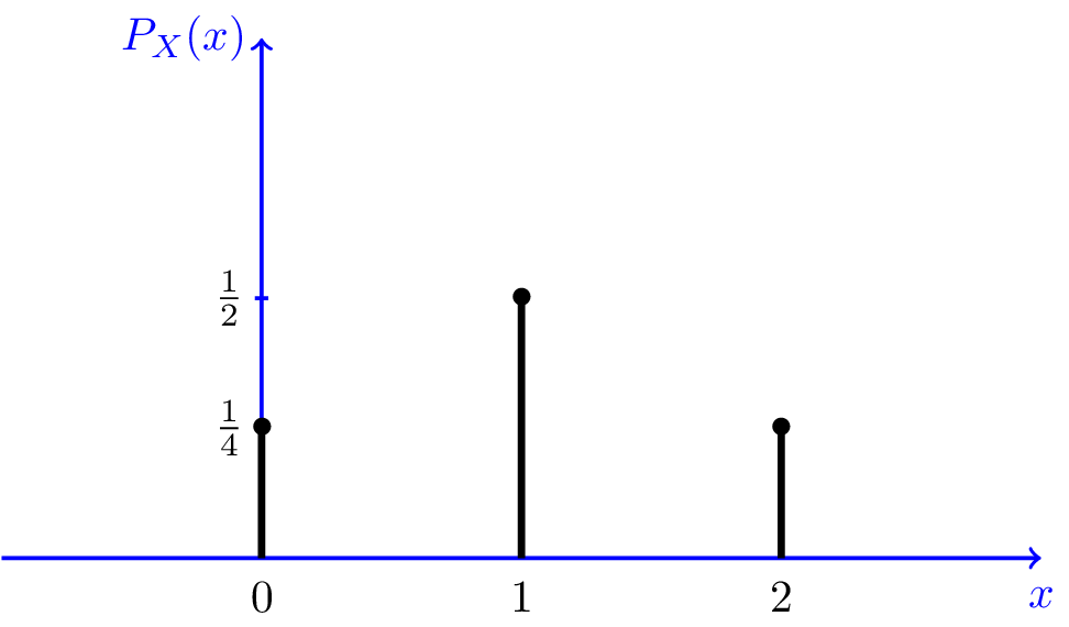
\[P_{X}(0)=P(X=0)=P(TT)=\frac{1}{4}\]
When k=1, meaning, we got one head, from our sample space this is possible by the following: HT,TH. Therefore the probability is:
\[P_{X}(1)=P(X=1)=P([HT,TH])=\frac{1}{4} + \frac{1}{4}=\frac{1}{2}\]
Finally for k=2, we get:
\[P_{X}(2)=P(X=2)=P(HH)=\frac{1}{4}\]
Visualy our PMF looks like this:
Lets drive the concept with a slightly more complicated example.
Ex: Consider an experiment where a fair coin is tossed over and over until heads is obtained for the first time. What is the probability of this event?
First lets look at some possible outcomes.
(H), X=1 … first coin toss results in heads.
(T,H), X=2 … second coin toss results in heads.
\(\underbrace{(T,T,T,T,…,T,H)}_\text{k-1}, X=k\) … kth coin toss results in heads.
If we say \(p\) is the probability of heads, then \((1-p)\) is the probability of tails. Then
\[P_{X}(k)=P(X=k)=P(TT…TH)=(1-p)^{k-1}p, k=1,2,…\]
Expected Value of a Random Variable
The expected value o a random variable X, denoted as \(E(X)\) or \(E[X]\) is a generalization of the weighted average, or the arithmetic mean of a large number of independent realization of X. The expected value is also knows as the expectation, mean, average, or first moment.
If \(f(x)\) is the pmf of a random variable X of the discrete type with space S, and if the summation
\(\sum_{x \in S}u(x)f(x),\) which is something written as \(\sum_{S}u(x)f(x)\)
exists, then the sum is called the expected value, and is denoted by \(E[u(X)]\). That is,
\[E[u(X)]=\sum_{x \in S}u(x)f(x)\]
Useful Facts
- If c is a constant, then E(c) = c.
- If c is a constant and u is a function, then
\[E[cu(X)]=cE[u(X)]\]
- If c1 and c2 are constants and u1 and u2 are functions, then
\[E[c_{1}u_{1}(X) + c_{2}u_{2}(X)]=c_{1}E[u_{1}(X)]+c_{2}E[u_{2}(X)]\]
Ex: You play a game and the rewards are as follows:
- You can win 1 dollar with a probability of 1/6.
- You can win 2 dollars with a probability of 1/2.
- You can win 4 dollars with a probability of 1/3.
How much do you expect to win on average if you play the game an infinite number of times?
\[E[u(X)] = 1*\frac{1}{6} + 2*\frac{1}{2} + 4*\frac{1}{3} = 2.5\]
Here we took the probabilities of the different outcomes and multiplied them by their numerical values (outcomes) and added them up.
This is a reasonable way to calculate the average payoff if you think of these probabilities as the frequencies of which you obtain the different payoffs.
It doesn’t hurt to think of probabilities as frequencies when you try to make sense of various things
Ex: Let a random variable X have the pmf
\[f(x)=\frac{1}{3}, x \in S_{X}\]
Where \(S_{X}={-1,0,1}. Let\ u(X) = X^2\). Then
\[E(X^2)=\sum_{x \in S_{X}}x^2f(x)=(-1)^2\frac{1}{3} + (0)^2\frac{1}{3} + (1)^2\frac{1}{3} = \frac{2}{3}\]
Variance of a Random Variable
A measure that determines the degree to which the values of a random variable differ from the expected value.
\[var(X) = E[(X - E[X])^2] = \sum_{x}(x - E[X])^2PX(X) = E[X^2] - (E[X])^2\]
Standard deviation
The square root of the variance.
\[\delta_{X}=\sqrt{var(X)}\]
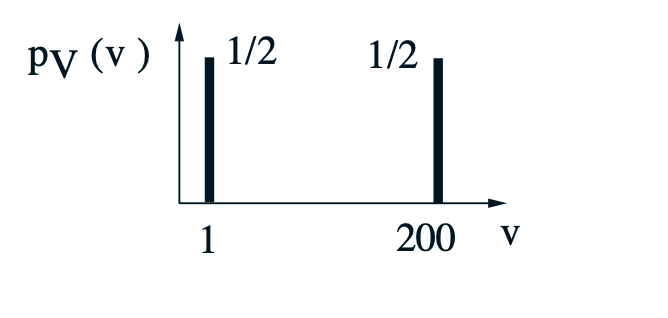
Ex: You need to traverse a 200 mile distance at constant but random speed V. You flip a coin, if its tails, you will walk at 1 mph. If its heads you take a plane that travels at 200 mph.
- You have 50% chance of going at 1 mph.
- You have 50% chance of going at 200 mph.
- Distance is 200 miles
What is the average speed at which you travel, the variance and standard deviation.
\[E[V] = \frac{1}{2}*1 + \frac{1}{2}*200 = 100.5\]
\[var(V) = \frac{1}{2}*(1 - 100.5)^2 + \frac{1}{2}*(200 - 100.5)^2 = 100^2\]
\[\delta_{V} = \sqrt{100^2} = 100\]
Time in hours = T = t(V) = 200/V, what is the average time?
\[E[T] = E[t(V)] = \sum_{v}t(v)PV(v) = \frac{1}{2}*200 + \frac{1}{2}*1 = 100.5\]
So if we were to run many itterations, on average it would take you 100.5 hours to travel 200 miles distance.
KL Divergence
Let’s say you have two coins, a Nickel and a Dime. They might be unfair (meaning that they might not be heads or tails 50% of the time).
You are running a gambling ring. People come up to you, and they bet on whether the Nickel will come up heads or tails when you flip it. If they bet a dollar per flip, how much should they win if they get it right?
You might think they should just win a dollar any time they are right, and lose a dollar any time they are wrong. But what if the Nickel is unfair? What if it comes up heads 80% of the time? Smart bettors will take a lot of your money by betting heads. So you might want to change the payout so that if they bet heads and get it right, they only win $0.25. And if they bet tails and get it right, they win $4. This way, on average, you will win as much as you lose. And the bettors don’t have an advantage or disadvantage by betting heads or tails.
What does this have to do with KL divergence? Well let’s say that you can’t flip the Nickel yourself to figure out how often it comes up heads. How do you decide what each bet should be? You could just default to the “bet a dollar, win a dollar” setup. Or you could flip the Dime. Let’s say that you flip the dime a thousand times, and see how often it comes up heads or tails. You could use the Dime to guess how the Nickel will behave.
KL Divergence is a measure of how “good” the Dime is at predicting what the Nickel will do. If the KL Divergence is 0, then the Dime is a perfect predictor of the Nickel - they both come up heads or tails at the same rate. But if the Dime is a bad predictor of the Nickel’s behavior, the KL Divergence will be large. This basically means that if you were using the Dime to make your decisions, and you replaced it by actually flipping the Nickel a lot and seeing what it does, you would gain a bunch of information and be able to set better odds (odds that don’t allow smart bettors to take your money).
More generally, KL Divergence says that if I use distribution A to predict the behavior of some random process, and the process actually happens with distribution B, how much worse am I doing by using A as an estimate than if I had access to B directly?
Sources
Resources used for this page